BCxA and NCBC

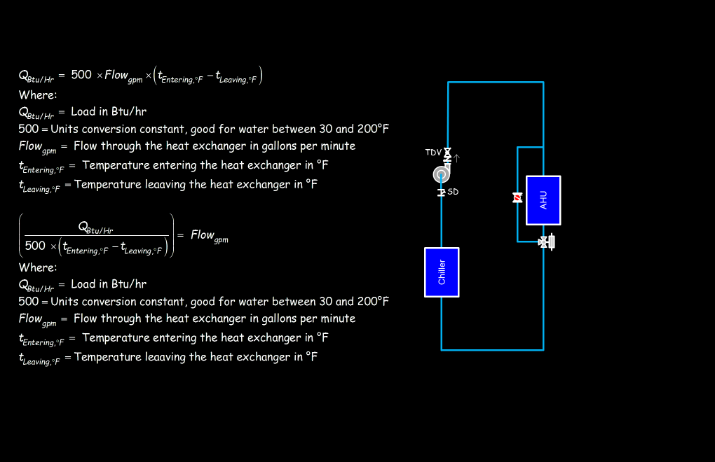
Building Commissioning Association and National Conference on Building Commissioning

The Building Commissioning Association Conference (BCxA) conference had its origins in the National Conference on Building Commissioning (NCBC). Thus, us older folk still seem to call it NCBC and even use that acronym for pages on websites, leading to confusion for younger folks. I here-by apologize for that and have made appropriate changes. I am still figuring out when that transition officially occurred so the buttons below are probably mislabeled to some extent, but I will get that fixed too eventually.

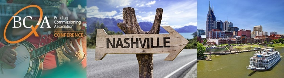
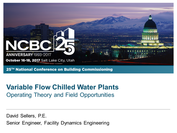
The following links will let you download files from/for various NCBC/BCxA conferences that I have presented at in one form or another. Note that there are some conferences where I presented but have yet to upload materials. All I can say is these thigns take time.

BCxA 2021 Workshop
Life Cycle Cost-Based Filter Operation Workshop
Class Materials

These are the files we will be working with in the class today.
PRESENTATION

2021_filters_final.pptx
File Size:	31049 kb
File Type:	pptx

FIRST GENERATION SPREADSHEET TOOL

ahu_2_filters_-_existing_and_summary_r1.xls
File Size:	1044 kb
File Type:	xls

ahu_2_filters_-_proposedr1.xls
File Size:	1589 kb
File Type:	xls

SECOND GENERATION SPREADSHEET TOOL

filter_loading_model_gen_2_v10_leconte_ahu2_orig.xlsx
File Size:	46112 kb
File Type:	xlsx

filter_loading_model_gen_2_v10_leconte_ahu2_orig_sched.xlsx
File Size:	43443 kb
File Type:	xlsx

filter_loading_model_gen_2_v10_leconte_ahu2_orig_sched.xlsx
File Size:	43443 kb
File Type:	xlsx

FILTER DATABASE

filter_loading_data.zip
File Size:	8011 kb
File Type:	zip

Follow Up Materials

Follow up materials for topics that come up in the session will be posted here with-in a week after the session.

BCxA 2020
Social Hour Presentation

mentors_life_and_cx_v4.pptx
File Size:	80280 kb
File Type:	pptx

These are the slides I used in the social hour presentation.

BCxA 2020
Preconference Workshop

The files below are the materials we will be working with in the preconference workshop. I will also put follow-up materials here after the class.

ballroom_ahu_v23_exercise_suv8.skp
File Size:	64341 kb
File Type:	skp

01_-_introduction.pptx
File Size:	80132 kb
File Type:	pptx

04_-_economizer_calculations.zip
File Size:	7313 kb
File Type:	zip

hru1-v5r2_-_kinematics_suv8.zip
File Size:	3707 kb
File Type:	zip

02_-_economizer_overview.zip
File Size:	12203 kb
File Type:	zip

05_-_07_-_pump_optimization.zip
File Size:	66138 kb
File Type:	zip

plant_v40_tour_suv8.zip
File Size:	76217 kb
File Type:	zip

03_-_economizer_evaluation.zip
File Size:	44491 kb
File Type:	zip

06_-_pump_head_estimate_v1.pptx
File Size:	9946 kb
File Type:	pptx

Follow Up Materials

The materials below are the follow-up materials I mentioned that I would provide. Please let me know if I have forgotten something. These files are my working spreadsheets etc. and they are somewhat complex. I am working on two blog posts that will cover the topics they address and have shifted them to the "top of the stack" given the questions from the class. Meanwhile, if you have a question about them, use the contact link to get in touch with me and I will set up a conference call to discuss it with you.

01_le_conte_annex_example.zip
File Size:	24123 kb
File Type:	zip

The files to the left have the savings calculations for a system on the UCB campus where we realized that the economizer dampers were oversized, and also not uniformly sized.

So we suspected that there would be poor mixing and also perhaps a surge in flow as the system went from minimum outdoor air towards 100% outdoor air. If you want to know more about the test data behind this, you will find it in this blog post.

This turned out to be true and the fan energy savings alone (there was also heating energy savings) easily justified the cost of a VFD to hold the flow steady. Once that was in place, it opened the door for other opportunities like zone level scheduling because the system runs 24/7 to serve zones on 2 of 4 floors that require that. The other two floors do not require 24/7 operation.

The reason I included this is to illustrate three things.

One is how you can use a field test at a couple of operating conditions to generate a mathematical relationship (in this case, a relationship between outdoor air percentage and system flow rate) that can then be used in a bin our hourly energy calculation to project annual savings.
The second is to illustrate how, in existing building commissioning, you often do not need to calculate all of the savings, just enough of the savings to get you the hardware and/or software you need to make an improvement. In this case, the fan energy savings (relatively straight-forward to calculate) justified the addition of a VFD for the supply and relief fan. Given the Owner's long term perspective (5-10 year simple paybacks), it also generated enough interest in the zone level scheduling opportunity to cause them to add dampers to the zone ducts that could be shut down. They also decided to upgrade the economizer dampers to eliminate damper leakage during a warm-up cycle and improve mixing.
The third is to illustrate how using an hourly calculation can improve your savings projection relative to what you can get from a bin calculation simply because of the added granularity it allows. In the olden days, repeating multiple calculations manually with a slide rule, calculator, and manual data entries from a psych chart 8,760 times was un-manageable, thus the evolution of bin calculations. But the formulas you use for the bin calculation and hourly calculation are identical. The only difference if you have a modern computer is the need to copy and paste them into 25-30 rows (i.e. 25-30 bins) vs. 8,760 rows (one row per hour).

02_typical_ahu_chw_load.zip
File Size:	39625 kb
File Type:	zip

03_chiller_plant_model.zip
File Size:	36871 kb
File Type:	zip

The files to the left are examples of how I come up with the theoretical chiller plant load profile cloud that I superimposed on the Atlanta Airport Marriot load profile cloud, which allowed me to identify load conditions were chillers were running when they should not have needed to run.

The general concept is to make some fairly general assumptions that are grounded in the characteristics of the systems in the facility you are looking at to "bracket" the possible conditions and then use an hourly weather data file (for instance one of the NREL TMY 3 data files).
The files in 02 Typical AHU CHW Load.zip are a very general case that looks at what happens with four 20,000 cfm AHUs in different configurations (100% OA, constant volume at design flow and economizer equipped VAV at design flow and 50% flow) to establish the theoretical cloud.

The files in 03 Chiller Plant Model.zip go a little further and look at the systems served by the chiller plant in the model, including the impacts of schedules, an estimated VAV load profile for the VAV systems, and an estimated base load.

BCxA 2019
Control System Fundamentals and Systems Logic Modification

The zip files below are the materials I provided prior to the class. They are the same materials as were on the USB drives I had in the classroom. If you page down a bit, you will find the follow-up materials I mentioned I would provide after the class along with a brief explanation of what each of them is.

Class Materials

logic_diagram_tool.zip
File Size:	2905 kb
File Type:	zip

bureacratic_affairs_building_scavenger_hunt.zip
File Size:	6936 kb
File Type:	zip

hx_logic_exercise.zip
File Size:	7234 kb
File Type:	zip

davis_hall_exercise.zip
File Size:	17389 kb
File Type:	zip

light_control_exercise.zip
File Size:	2120 kb
File Type:	zip

level_control_exercise.zip
File Size:	28832 kb
File Type:	zip

two_third_rule_model.zip
File Size:	13876 kb
File Type:	zip

pdf_presentations.zip
File Size:	17900 kb
File Type:	zip

Follow-up Information

04_-_control_processes_v3.pptx
File Size:	12163 kb
File Type:	pptx

The PowerPoint file to the left is a version of the slides I did on PID that is the "full meal deal" and includes information on:

How one and two pipe pneumatic controls work and some of the pros and cons of pneumatics and pneumatic actuation vs. DDC,
Floating control, which is a less common type of proportional control process but useful for some applications,
What the "I" and "D" gain engineering units mean,
PID tuning,
Lags and their impact on control process tune-ability,

There are animations on some of the slides that help convey concepts, so you may want to actually run them as a slide show vs. viewing the in the editing mode. Note also that there are some PID resources on a different page of this website that you may find helpful.

And the current plan is to have the "full meal deal" PID lecture recorded in a month or so as a series of "bite size modules that you could watch on a break or something (because who would want to go out for a walk on a nice fall day when they could watch a thing on PID). So you may want to check back on the PID resources page if that sounds like something you could use to cure insomnia or something.

02_level_control_logic_value_added.pptx
File Size:	17768 kb
File Type:	pptx

The presentation to the left contains the slides I used in class to illustrate the value of picking up an overflowing cooling tower; basically, a little bit over a long time is a lot.

03_-_reset_schedule_information.zip
File Size:	667 kb
File Type:	zip

The zip file to the left contains a number of items including

An e-mail I wrote to one of the folks in a Marriott training class to describe how to do a reset savings calculation.
An example of how significant the savings can be from reduced operating temperatures, even if a pipe is insulated.
The finned tube performance graphs we were looking at in class.
An example of a reset savings calculation using bin data. An hour by hour example would use the same approach and formulas.
A tool I use to figure out the y=mx+b equation for a reset schedule and then document how well it is working out in the field.

The image to the left is the three-way switch logic option that Treasa shared in the class. The PowerPoint below is the light switch ladder diagrams with the dimmer diagram modified to show the on-off function as suggested in the class. The Excel file is the Logic Diagram tool I was using in class for the interactive stuff we did.

05_-__three-way_switch_v2.pptx
File Size:	265 kb
File Type:	pptx

logic_diagram_tool_class_workbook.xlsm
File Size:	1680 kb
File Type:	xlsm

The "answers" the the heat exchanger control process in terms of adding some enhancements are at this link. In addition to the heat exchanger logic (shown to the left), you will find examples of some of the other logic associated with the HHW pumps, like the start-stop/lead-lag logic and the logic that controls the finned tube, both before and after the EBCx team finished their work.

I realized after the class that I had tabled a question for further discussion later

but then, we never actually had the discussion. So I am in the process of making a string of informal videos that walk through the logic and describe how it works in general, including a discussion about how and why to cap reset schedules, which is the question that I tabled and forgot.

07_-_tab_04.6_-_physical_and_code_and_terminal_strips_v4.pptx
File Size:	45514 kb
File Type:	pptx

Finally, the slides to the left are the ones I mentioned that provide more detail on the specialty terminal strips that I gave an example of in the class.

NCBC 2018
Assessing and Optimizing Central Chilled Water Plant Load and kW per Ton Profiles

Years ago, after doing my very first load calculation (which was a manual effort based on a myriad of tables, charts and equations back in those days) I found myself sitting across the desk from Bill Coad as he reviewed the results of my efforts. After looking things over and asking a few questions, Bill said something that total baffled me until he explained himself.

Nice job David; that’s the most useful, meaningless, piece if information we will develop for this project.

How can something be useful and meaningless at the same time I found myself wondering?

Sensing my confusion, Bill went on to explain what he meant. Specifically, he explained that we would be using the design load I had just calculated to select the various pieces of equipment for the project. And that single number would also set the size of the distribution systems the machines would serve as well as the size of the utility systems serving the machinery. And financially, all of those things would eventually set the project budget. Thus, getting the design load right was critical to success in all of those areas.

  But ...

Bill continued while keying a few numbers into his HP calculator,

... there are only a handful of hours a year at the conditions behind all of that math you just did;
  350.4 hours to be exact. Fewer actually, because some of those hours will be above the number
  we are hanging our hat on.

Thus began my fascination with load profiles and part load efficiency and performance. And what I hope to do in this class is share some of that fascination with you, along with the lessons Bill and other mentors (including machinery and buildings) have taught me.

  Commissioning is a process during which buildings mentor us about our designs.
Me
Part of the plan is to work a tour of the central chilled water plant serving the conference location this year, none other than the 10,000 ton plant serving the Gaylord Opryland Resort & Convention Center. The idea is to spend some time ahead of the tour sharing ideas about what drives a load profile for a chilled water plant and how the machinery typically found in a central plant responds to those drivers so that by the time we go into the plant, you will be "primed" to see it in a different way.

I actually won't get to see the plant myself until the Friday before the conference and as a result, the agenda for the class is still in a bit of a state of flux. But having said that, here is what I think we will cover over the course of the day; basically, my working agenda for the class.

Load Profile Drivers
Developing a Load Profile
Chilled Water Plant Machinery (Motors, Pumps, Pipes, Refrigeration Equipment, Heat Rejection Equipment, Heat Transfer Equipment)
Distribution Strategies
Comparing a Centrifugal and Absorption Chiller
Tailoring the Machinery to the Load Profile and Rate Structure
Central Plant Design Case Study

I'm hoping to make the class fairly interactive, including potentially working with you in Excel to illustrate basic techniques that you might find useful for doing an assessment of a plant. So, while you don't absolutely need to have a laptop or Excel skills for the class, you may find it helpful to bring your laptop if you want to work along.

And don't let a lack of Excel skills scare you off. Part of how you learn to do things with Excel is by trying it and we plan to have a few "floaters" in the room who can jump in if you are not quite following. Plus, we will encourage you to work in teams for the exercises so you can always team up with an Excel savvy neighbor and work on things together. You may even want to line such a partnership up ahead of time.

In terms of other things you might want to do to get ready, time permitting, here are some suggestions. Since part of the "trick" in working with load profiles is understanding the machinery that is doing the work, you may want to "bone up" on pumps, chillers, and the other items mentioned in the Chilled Water Plant Machinery bullet above.

One resource that you might find helpful in that regard is the Resource List we provide here on the website. Its fairly well bookmarked and you will find quite a few relevant resources under the Centrifugal Machines and Refrigeration and Cooling Equipment topics. You will also find some information on induction motors on the Induction Motor Principles page of this web site.

I also help support day long classes at the Pacific Energy Center on topics like Pumps and Piping, Chilled and Condenser Water Systems, and Variable Speed Drive. All of the materials from those classes can be found on the Pacific Energy Center Classes page of this website.

And I will sometimes reference common HVAC equations for energy and load (yes, there is math involved). I have been building web pages for the more common formulas like the square law and the equation for pump power and energy. So you may want to reference them before or after the class. There is also a page with a PowerPoint I use that has most of the common equations in it along with a number of other useful HVAC relationships and concepts.

But even if all you did was show up for the class with an open mind and some curiosity, I would like to think you would benefit from it. If nothing else, you will get to see a really big chilled water plant, something most folks in our line of work would find to be quite informative and enjoyable.

So, bottom line, as I finalize the content for the class, I will be posting it here, starting on Saturday some time and continuing through the weekend as I get all the i's dotted and the t's crossed. So, if you are taking the class, you probably will want to check back here every-once-in-a-while, or at least on Monday morning before heading down to the class room to pickup the content. I will also post follow-up materials here after the class.

See you next week,

Class Materials

These are the materials for the class tomorrow. There are a lot of files; some of which are somewhat large.

Don't panic; stay calm and continue to breath normally.

There are a lot of resources included in this. Truth be told, I think you will do just fine if you come to the class and just watch what I do and participate in the lab session, perhaps occasionally partnering up with your neighbor when I am doing something in Excel interactively.

But, based on past experience, quite a few people find the details useful, thus I have included them.

See you in the morning; the plant we will visit is "way cool".

class_materials_-_part_01.zip
File Size:	190384 kb
File Type:	zip

class_materials_-_part_02.zip
File Size:	204912 kb
File Type:	zip

class_materials_-_part_03.zip
File Size:	211314 kb
File Type:	zip

class_materials_-_part_04.zip
File Size:	54688 kb
File Type:	zip

class_materials_-_part_05.zip
File Size:	114081 kb
File Type:	zip

class_materials_-_part_06.zip
File Size:	9261 kb
File Type:	zip

NCBC 2017
Variable Flow Chilled Water Plant Workshop - Preclass Materials

The Variable Flow Chilled Water Plant workshop will rely heavily on interactive exercises using Sketchup Models. To maximize the benefit of attending the workshop, I highly recommend you bring a laptop to the session and download and install the free version of Sketchup (Sketchup Make) if you do not already have it on your laptop. You will find information on how to go about doing that on the Sketchup Models page of this website.

With the release of the latest version of SketchUp, the program no longer supports computers with 32 bit operating system in order to fully leverage the graphic capabilities of the current technology. But not everyone has a 64 bit computer. To address that, I have uploaded the install files for a number of older versions of SketchUp on the SketchUp page of the website.

The models we will use in class can be downloaded by selecting the file below. It contains four different models:

A model of a central chilled water plant.
A model of the cooling towers serving the plant and the site that the central chilled water plant is located on.
A model of an air handling system that is one of the loads on the central chilled water plant.
A model of the duct system and area served by the air handling system.

We will work primarily with the chilled water plant model but will likely also use the others as a part of the class activities depending a bit on where your questions take us.

The models have been back-saved as SketcUp version 8 files to ensure they will open with older versions of SketchUp. So they should work with any version of SketchUp from Version 8 forward. If you open them in a newer version, you will get a little warning telling you that the file was created in an older version and that if you save it, it will be converted to the format associated with the version of SketchUp you are running. All you need to do is acknowledge that.

NCBC Variable Flow Chilled Water Plant Workshop Models (ncbc_2017_variable_flow_chw_plant_workshop_sketchup_models.zip)
File Size:	81798 kb
File Type:	zip

Variable Flow Chilled Water Plant Workshop - Follow-up Materials

What follows are the slides and other materials I used as a framework for the class session. Since the class is, by design, somewhat free-form, I usually have a lot more material on hand than I will actually use. What I use depends on where the interactive discussions take us. So, in what follows, I have included items I had "on deck" to use depending on how the session flowed in addition to information that supports the topics we discussed. I offer all of it as additional information and it is what it is. You can always get in touch with me if you have questions.

Main Module

Pumps

Variable Flow Evolution

System Diagram Answer

Slides

These are the slides I used as a framework for the class yesterday. Because they were a framework rather than a formal presentation, you will notice that I did not present them in the same order nor did I present all of the slides. Because of color pallets and slide size, the slides are actually spread through a main module and three sub-modules that are linked to the appropriate slides in the main module.

Slides I didn't cover directly include:

Slides 77 - 79 - These take a closer look at the instrumentation we installed to develop the load profile for the Seattle high-rise I was using as an example. I have included the informal pricing documents we used to get the sensors installed in the supplemental information that follows along with a bit more of a description of why I think it is relevant.
Slides 80-84 illustrate how we used the data we collected to develop the plant load profile. The spreadsheets behind them are included in the supplemental information that follows along with a few comments on why they are relevant.
Slide 85 is the kW per ton profile for the plant design plotted against the load profile. The spreadsheet behind that is included below along with a bit more of an explanation about why it is relevant.
Slides 86-87 illustrate a technique based on a simple test and basic data loggers that can be used to develop a plant load profile for a plant like the one in the model.

Variable Flow CHW Class Slides (ncbc_2017_variable_flow_class_slides.zip)
File Size:	74513 kb
File Type:	zip

Pump Design Briefs

The file below contains the two Energy Design Resources Design Briefs I mentioned on the topic of pumps. If you want to know more about pumps, you may also find the materials from the Pumps; Design, Performance and Commissioning Issues class I present with Ryan Stroupe at the Pacific Energy Center to be of interest.

Energy Design Resources Briefs (edr_pump_design_briefs.zip)
File Size:	3579 kb
File Type:	zip

Plant Evaporator Pump Optimization

As we discussed, two of the opportunities in the central plant model were related to the evaporator pumps; one of them was in "Hand" and both of them had their discharge valves throttled. We discussed the savings assessment for those items generally in class. The spreadsheet below has the analysis and calculations included in it.

It was built using the Plot Digitizer Pump Curve Example spreadsheet as a starting point, modifying the data that was generated using Plot Digitizer to reflect the evaporator pump curve, and then performing the analysis to compare throttling to a speed reduction and an impeller trim.

The benefit of using a digitized pump curve is that since the impeller curves associated with different impeller sizes and speeds and the system curve are all mathematically defined by the affinity laws, you can quickly plot them by doing the math in a table vs. manually plotting points.

The spreadsheet has:

Tabs with the data that create the pump curve (red); the resulting curve was simply copied and used multiple times for the rest of the analysis.
Tabs that generate the design system curve (orange)
Tabs that generate the design impeller line (yellow)
Tabs that generate the wide open system curve (green)
Tabs that generate the line for the trimmed impeller option for saving energy (blue)
Tabs that generate the impeller line for the reduced speed option for saving energy (purple)
Tabs with the savings calculations for the pump optimization and having the Hand-Off-Auto switch in "Hand" (black)
Tabs with the TMY3 weather data used in the savings calculations (white)

Note that the savings calculations have been done for four different locations and how the results vary significantly due to the nature of the climate, the utility rates and the desired plant operating sequence (the pump serves the lead chiller and the result would be different if it served the lag chiller).

evaporator_pump_optimization_calculations.xlsx
File Size:	3394 kb
File Type:	xlsx

Plant Distribution Pump Optimization

There are several findings that you could identify in the chiller plant model related to the distribution pumps including throttled triple duty valves, VFDs in hand and at full speed and what seems like a fairly high differential pressure set point for the current operating condition.

If you looked at the AHU model as being representative of a load on the system at the end of the line, you would discover that the chilled water valve is throttling pretty hard (more closed than open if you climb up the ladder and take a look), even though there is obviously flow through the coil (condensation, pressure drop and temperature change on both sides).

You also may have noticed that there is a differential pressure transmitter piped across the pump header at the central plant that appears to be the input to the control process setting the pump speed. As a result, you may conclude that you should investigate some sort of reset schedule that resets the set point of the control process based on what is going on out in the system; basically, leverage the two-thirds rule.

If you really dig into that a bit, you will also discover that the distribution pumps are best first cost pumps not best life cycle cost pumps. The original selections were best life cycle cost but were Value Engineered (VEd) out of the project as can be seen from the equipment schedules on the plan table (tab 46 in the model).

The spreadsheets in the zip file at the end of this section illustrate the analysis you might do to explore different ways to achieve savings including optimizing the existing pumps via number of ways and upgrading the pumps to more efficient selections and optimizing the speed control for them. The model is base on an actual flow profile from a smaller plant.

Flow Profile v2.xlsx Spreadsheet

The results of the analysis are in the Summary tab.
The Data tab takes the original load profile and shifts it based on the plant tonnages. It also calculates the chiller starts and hours that show up on the chiller displays.
The Flow tab generates the flow profile for the model plant based on the shifted load profile and then calculates the energy savings for a number of ways of controlling the secondary pump differential pressure.
Note that using a trim and respond approach applied to the existing pump generates more savings for much less cost than upgrading to a significantly more efficient pump but using a less ideal speed optimization strategy. Of course the most efficient pump plus the trim and respond optimization would yield the most savings if you had the money and the control network would support the traffic required for trim and respond. But the point of the exercise I use this data for is that many times you can get a significant chunk of the ideal savings simply by optimizing a control strategy.

Bhp vs Flow 1510 ... Spreadsheets

These spreadsheets are based on a technique I use to come up with a relationship for pump energy as a function of flow for a given system. I developed it because I concluded that using the SCE affinity law coefficients that are typically used (see the file associated with the Affinity Law Exponents section below) would tend to over-state the savings if the plant had a lot of part load hours. The reason I concluded this is that those coefficients will project that the pump energy at 0 gpm is 0 kW, which is not the case for a real world pump; just think about dead-heading a pump. The flow is in fact forced to 0 gpm, but the pump, of course, is still spinning and drawing power.

How important this distinction is will depend on how many part load hours the plant has and the tonnage at those part load hours. If the plant runs fully loaded most of the time, it is not as critical as if the plant spent a lot of hours at part load. But there are quite a few plants that have a significant number of their hours at low load conditions. For example, I was just working with a team on a 700 ton plant that spent 90% of its time at or below 200 tons and 80% of its time at or below 140 tons.

The approach I use is based on the pump curve and affinity laws. Having the ability to digitize a pump curve makes it really fast; much faster than if you hand plotted the various system curves on a pump curve manually. Tim precludes writing a detailed description currently; probably a good blog post. But you can probably reverse engineer what I do from the spreadsheets if you need to. The basic steps are:

Digitize your pump curve and get it into Excel using Plot Digitizer. I have a page on the web site that hooks you up with Plot Digitizer and also gives you a digitized pump curve that you can use as a starting point if you want to try this. (red tabs in the spreadsheets)
Plot the design point system curve. (orange tabs in the spreadsheets)
Estimate the pressure drop from the pump location to the point in your system where you are measuring and maintaining a fixed pressure. The technique assumes your control process will hold a fixed pressure at some point in the system. So that pressure will never vary but the pressure drop from the pump to that location and back will vary as the square of the flow.
Reduce the flow rate by some arbitrary amount. I usually do 75%, 50%, 25% and 12.5%. The more points, the better the curve fit when you project the flow vs. pump energy line so this is a trade off between curve fit and engineering time to develop it.
Calculate the head required at this new flow rate based on the fixed head you will maintain at the sensor location and the portion of the design head that will vary with flow in the piping between the pumps and the sensor location.
Use the square law to project a system curve through this point and read the efficiency where it crosses the design impeller line. This is the efficiency you will use in your pump power calculation at the reduced speed since reducing the pump speed moves you up and down a system curve and preserves the pump efficiency.
Use the speed affinity law to project the pump speed and impeller curve through the new operating point. (yellow tabs in the spreadsheets)
Repeat steps 4-7 for each of the flow reductions you want to assess. (green, blue, and purple tabs in the spreadsheets)
Plot your data points as pump power (y) vs. flow (x) and use the Excel trendline feature to develop an equation that lets you calculate the pump power for a given flow condition (black tabs in the spreadsheet).
Use the equation you developed along with the flow profile to calculate pump power for a given flow condition (the blue, purple, orange and red columns in the Flow tab of the Flow Profile v2.xlsx spreadsheet.)

The Affinity Laws Speed - Case 1 Details v2.pptx file illustrates these steps. The summary tab of the Bhp vs Flow 1510 5E 1750 rpm Remote DP.xlsx spreadsheet compares the results associated with the analysis in that spreadsheet with the results from the other options on the summary tab starting at line 41.

DP Sensor Addition v1.xlsx, Trim and Respond Programming v1.xlsx, and Adding A Pump v4.xlsx Spreadsheets

These spreadsheets are the cost projections associated with each of the options I looked at for optimizing the distribution pumps in the central plant.

Distribution Pump Optimization Example Files (distribution_pump_optimization_example.zip)
File Size:	12591 kb
File Type:	zip

Affinity Law Exponents

The affinity laws state that pump energy varies as the cube of the flow rate and there is a temptation to calculate pump and fan power for variable flow systems based on this relationship. However, the relationship is based on a fixed system curve and variable flow systems actually operate on a family of system curves.
In other words, every time a valve or damper moves, it establishes a new system curve. So the power consumption for the system will approach the cubic relationship but not match it.

At one point, Southern California Edison funded some research to establish exponents that could be used to project pump energy savings for different sensor locations in a variable flow system. But those exponents will tend to overstate the savings if a plant spends a lot of time at part load, as I mentioned above.

The zip file below includes a spreadsheet that compares the various SCE exponents and has a tool in it that helps you estimate an appropriate exponent for your system from the SCE data based on the design operating pressure for your system and the pressure you will maintain at the controlling sensor location using a variable speed drive.

It also includes the original SCE technical bulletin that published the exponents and recommendations on how to apply them.

Spreadsheet Tool for Estimating a Flow vs Pump Power Exponent (affinity_law_exponents.zip)
File Size:	210 kb
File Type:	zip

Variable Flow in Condenser Water Systems

Davis Hall Example

I used the Davis Hall condenser water system to illustrate how the variation in head requirement that occurs at different flow rates in systems with long runs of common piping can cause a constant flow system to actually be a variable flow system.

The zip file to the right contains the model I used along with the system diagram and a presentation I use that illustrates the results of the testing we did on the system that documented the issue.

David Hall Example(davis_hall.zip)
File Size:	11182 kb
File Type:	zip

The Impact of Flow Variation Over Towers on Tower Flow Distribution

One of the things I had "up my sleeve" that we did not get to in the class was the impact of flow variation over a tower on its performance. It turns out that if you reduce the flow too much for a given tower, then you will no longer wet all of the tower fill. If you don't wet all of the tower fill, air will short circuit around the fill since it is easier for the air to pass through the dry fill relative to the wet fill.

If that happens, then the near linear relationship between tower fan energy and heat rejection is broken and the tower will use more energy that you expected for a given load condition. You can also start to deposit scale on the tower fill, even if the water quality is good, because on some of the fill, all of the water evaporates before it reaches the cold basin.

The reason this matters is that in the drive for energy savings we are implementing measures that will cause flow to vary over the towers. Two common examples are varying flow to manage head pressure, which was mentioned during the class, and opening more cells than you might need for the current load condition to spread the flow out and leverage the cube rule to save fan energy.

Both of these approaches will in fact save energy, but only if the tower performance is not degraded by poor flow distribution over the fill. I am about to publish a blog post that illustrates this and provides video clips that show the phenomenon happening in a number of towers. So rather than try to include that information here, I will suggest that you watch for that information to show up on my blog and on the videos page of the website.

2017-10-17
I am still working to get the supporting materials content on the site. I decided to put some explanatory notes in for each of the files so you would better understand what it represents and that its taking a bit of time. I will be attending sessions at the conference a lot today but will work on it during breaks and this evening and ultimately hope to finish by tomorrow evening if not sooner.

Low Delta-T Syndrome Example

We discussed Low Delta-T Syndrome or the "Death Spiral" in class a bit. In fact, if you look at what is going on in the plant in the model, it is in early Low Delta-T Syndrome; the supply and return temperatures to/from the loads are identical to the supply and return temperatures at the active chiller.

That means that the flow to the system is nearly the same as the flow through the chiller (1,100 gpm based on the evaporator pump nameplate if you assume the discharge valve was throttled to deliver design flow).

But, if the load on the plant is in the 250 - 350 ton range based on the various clues about that in the plant (its about 330 tons if you assume 1,100 gpm through the evaporator and that the temperature transmitters are accurate), and if its a 12°F delta t plant (550 ton chillers with 1,100 gpm flowing in the evaporator) then the actual system delta t of 7°F is low relative to the 12°F design condition. The primary reason for the lower than design temperature rise on the system side in this case is the performance of the cooling coils with non-design entering air conditions; they simply can not generate the design temperature rise with cooler, dryer air entering them.

The file below is just data from a plant that was in low delta-t syndrome for a number of days during the logging interval so you can see what that looks like in a real world situation. The plant was an nominal 2,400 ton, 16°F delta t plant serving a high rise office building in Seattle.

Low Delta-T Syndrome Example (2015-12-10_low_dt_v12.zip)
File Size:	16173 kb
File Type:	zip

Cooing Coil Model

We discussed how much cooling coil performance can vary with load conditions during class. As we saw, that works against the theoretical constant system temperature rise that is implied by a variable flow plant design. The implication is that by design, variable flow plants will drive into low delta-t syndrome unless the plant design takes the phenomenon into account. The files below are the Greehheck coil models I used to generate the data I presented along with the Excel file that contains the data and generated the chart to the right.

Cooling Coil Model Files (cooling_coil_model.zip)
File Size:	891 kb
File Type:	zip

Load Profile Example

During class, we discussed how important it is to understand the seasonal and daily load profile on the plant and then tailor the selection and operation of the equipment to that in addition to being able to meet the design load on the design day. The spreadsheets in the zip file below are associated with an analysis of a plant that was being designed to replace an aging plant in the high-rise that the low delta t syndrome data is from.

In the image above the building load profile is represented by the blue bars. The load profile was developed from measured data from the building; i.e. the building told us the load profile it sees. In this particular case, note how the plant actually can see hours at 2,400 tons but spends the majority of its time at or below 400-600 tons.

Based on this, the new plant was configured to include a 300 ton modular chiller and two 1,000 ton modular chillers. If the plant had been staged per the design sequence, the kW per ton profile would have looked like the red line because the original sequence ran the small chiller up to the point where it was nearly fully loaded before staging on a larger chiller.

Intuitively, that seems correct, but when you look at the chiller compressor kW per ton profile, you discover that the larger machine is actually more efficient than the smaller chiller at around 130 tons. If you take the condenser pump energy into account (the next largest component contributing to the over-all kW per ton profile) the larger machine is more efficient than the smaller machine at around 190 tons.

By staging the larger chiller on sooner, the kW per ton curve for the plant is shifted from the red line to the yellow line, improving the over-all efficiency at a point where a lot of operating hours will occur. A similar analysis suggested that staging the small machine back on as the second chiller instead of the larger machine would improve the over-all plant efficiency (the green line).

The point of all of this in the context of the class and existing building commissioning is that extracting the building load profile from actual building operating data and developing the plant kW per ton profile based on the characteristics of the installed equipment (or the proposed equipment in the case of a new plant) and then overlaying those to profiles can provide powerful insights into the best way to operate the plant. Frequently, improvements can be achieved by simply modifying the plant sequencing strategy.

The files in the zip file below are the files behind the chart at the beginning of this section. If you open them, they will probably seem complex. But if you take them one tab and one row at a time, I think you will discover that they are not as complex as they seem. The idea is to show you the techniques I use so you can revers engineer them and replicate the ideas on your own.

2016-07-05 Tons vs. OAT Tool v2.xlsx takes the logged data from the plant and generates the regression that projects plant tons as a function of outdoor temperature.
Load Profile Generator v3.xlsx takes the data from 2016-07-05 Tons vs. OAT Tool v2.xlsx and develops the load profile for the plant.
2016-06 CD kW per Ton v5 - 01 Per Sequence.xlsx develops the plant kW per ton profile and overlays it on the load profile. The chart at the beginning of this section comes from this spreadsheet.
Sensor Addition Drawings v4.pdf is the informal contract document we used to get the sensors in place to develop the building load profile. Note that we only needed the system temperatures and flows to develop the load profile. The other sensors were installed so we could develop energy savings projections for the new plant relative to the existing plant.

Load Profile Example (load_profile_example.zip)
File Size:	88523 kb
File Type:	zip

NCBC 2016

Under Construction; Coming Soon.

NCBC 2015

Filtration is an essential element of any HVAC process with some sort of filter found in virtually all AHUs. When one considers that at least one 2’ x 2’ filter will be required for every 2,000 to 4,000 square feet of building area and that CBECs data suggests that there are 58,800,000,000 square feet of commercial building space, then the number of filters associated with commercial HVAC systems is astounding. These figures do not include health care and process facilities, where filtration requirements are more stringent and multiple filter banks are common.

The operating cost for a given filter bank includes a first cost associated with the cost to procure/install the new filters and remove/dispose of the old filters. This tends to decline with time in service.

It also includes n operating cost associated with moving air through the resistance associated with the filters. This tends to rise with time in service. While it is not uncommon for filters to be changed based on time in service. However, if one considers that:

The nature of an HVAC process (e.g. 100% outdoor vs. economizer),
The operating hours (e.g. scheduled vs. 24/7),
The nature of the contaminant (e.g. cotton wood seeds vs. desert sand) and
The nature of the climate (e.g. rural vs. urban)

... will all likely impact the type and quantity of contaminants handled by the system, one will conclude that there is more than time in service to consider when contemplating the best time to replace filters for a given HVAC system.

This presentation uses a case study approach to discuss and explore operating filters on a life cycle cost basis v.s. time in service. The presentation will include data from systems where alternative technologies were operated side by side in identical systems over a period of years while data was logged on a 15 minute basis to allow the alternative approaches to be contrasted.

In one example, the more costly, best life cycle cost technology with a projected 42 – 48 month best life cycle cost took two years to reach the pressure drop associated with the alternative, legacy technology. In another case study, the more costly, lower life cycle cost approach exceeded the 42 month best life cycle cost projected by the model that drove the decision to try it out.

One of the keys to success with this approach is to recognize that filters with identical MERV ratings can have radically different performance characteristics. Typically, more highly engineered media, while having a higher first cost, will provide lower initial pressure drops, flatter pressure drop vs. dust load curves, and higher dust holding capacity relative to the lowest first cost technology.

As a result, the higher first cost technology often represents the best life cycle cost, saving fan energy, installation labor, and filter first cost and disposal cost (i.e. less to the landfill) making life cycle cost based filter operation attractive from a sustainable operations standpoint.

The download to the left is the PowerPoint presentation associated with this topic from NCBC 2017. The download to the right is a paper I published with Mike Chimack at ACEEE 2000 that is a case study of applying the concept in an operating facility. You will also find a number of posts on my blog that cover the topic starting with a post titled Demonstrating HVAC Filtration Savings with Data Loggers.

filters_finalr1.ppsx
File Size:	24402 kb
File Type:	ppsx

aceee_final_draft_paper_-_filters_-_for_distribution.pdf
File Size:	116 kb
File Type:	pdf

NCBC 2013

These are the materials associated with a presentation I did about writing a functional test for an EBCx/MBCx project. The presentation centers around a case study of the chilled water system in Le Conte Hall at UC Berkeley.

The system had a short cycling problem related to a new research load that was added and by using a functional test to ask the building about the dynamics of the load, we were able to learn enough to develop a flywheel cycle that solved the problem. The fix also allowed us to save energy via implementing an integrated economizer cycle on an air handling system that up to that time, used a non-integrated economizer cycle to prevent short cycling of the compressor in the air cooled chiller serving the system.

Writing a Functional Test (writing_a_functional_test_-_final_-_print.pdf)
File Size:	8012 kb
File Type:	pdf

leconte_chilled_water_system_v2.pdf
File Size:	430 kb
File Type:	pdf

Le Conte Chilled Water System Tests (le_conte_mbcx_tests_-_chw_system.pdf)
File Size:	79 kb
File Type:	pdf

I recently made a four module video series that includes this case study as well as a more comprehensive look at functional testing and uploaded it to the Introduction to Functional Testing page of the website. In addition, if you are interested in what the control logic modifications we made to implement the flywheel cycle looked like, they are included on the Eikon for Educators and WindLGC page of the website. The sample Eikon program that is provided there for you to "play with" is the logic modification we made.

NCBC 2009

This is a presentation I did for NCBC that uses a case study from one a "significant emotional event" early in my career as a way to illustrate some important technical lessons as well as some important lessons about mentoring and human interactions.

Mike Kaplan co-presented with me and also offered some very insightful, non-technical perspectives on managing some of the feelings and thoughts that might come up out as you work on a project that really complemented my presentations nicely so I have also included his paper.

mentoring_field_technicians.pdf
File Size:	2525 kb
File Type:	pdf

mentoring_pp_presentation.pdf
File Size:	2051 kb
File Type:	pdf

zen_and_the_art_of_cx.pdf
File Size:	103 kb
File Type:	pdf

NCBC 2007

This is a presentation I did for NCBC about my perspectives as a mechanical engineer on power failure and recovery from power failure.

An unexpected power failure and the ensuing recovery can wreak havoc on a building and its systems, generating complaints, loss of environmental control, quality control problems, and occasionally, debris. This presentation uses a case study format to illustrate and discuss important HVAC and building system considerations that should be targeted when assessing and testing the ability of a building and its system to recover from a loss of electrical power as well as other utilities.

me_perspective_v2.pdf
File Size:	4080 kb
File Type:	pdf

At the time I did the presentation, I had just helped PECI write the Integrated Operation and Control and Power Failure Recovery section of the Functional Testing Guide. (Note that the Power Failure Recovery link downloads the Word document vs. opening a new window). The guide is still up and running but given the age of the HTML, it will run better in Windows Explorer than the current browser assortment. I personally run it under Windows Explorer 11 and turn on compatibility mode.