The Affinity Laws
|
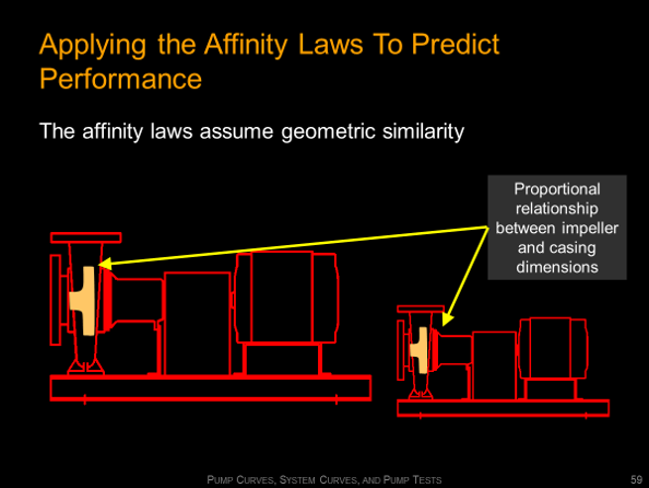
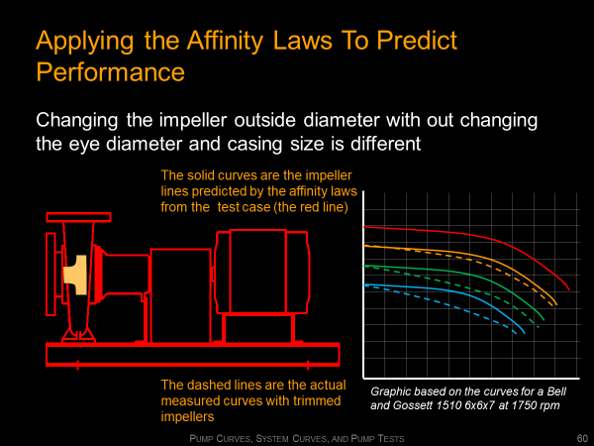
This page provides information and resources regarding the affinity laws that are used to project new performance points and curves for a pump or fan given a known performance point or curve. In general, the affinity laws project the new operating point(s) by moving up and down a system curve. That means the affinity laws can only be applied to a fixed system, which is an important constraint to recognize if you are going to use them.
For each of the laws listed below, you will find an explanation of how to apply them along with the equations from Mathtype in .wmf and .pdf form so you can document your math when you apply the concepts in a spreadsheet, which I believe is a professional and important thing to do. If you follow the link above, in addition to explaining my philosophy on this, it will also explain how you can use the equation files.
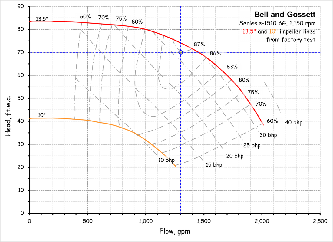
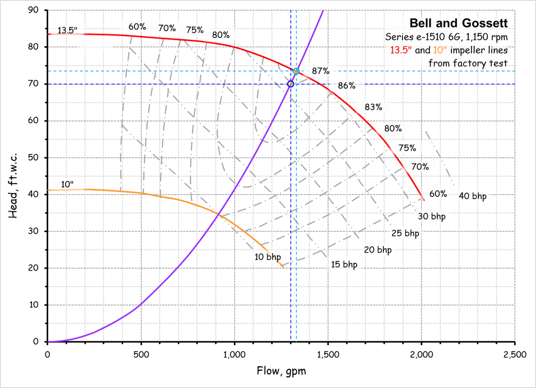
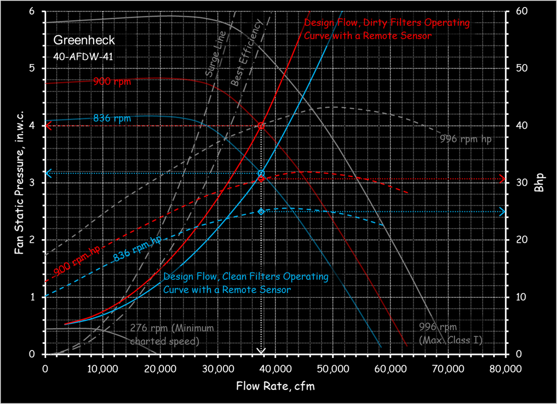
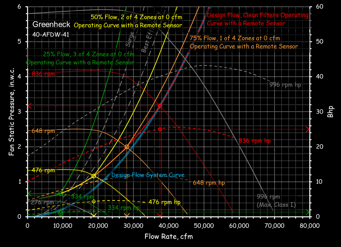
I have also included the spreadsheets that I used to generate the pump curve illustrations. They are based on the Plot Digitizer Pump Curve Example spreadsheet and illustrate how you can don the affinity law math in the spreadsheet and plot the result on the pump curve.
For each of the laws listed below, you will find an explanation of how to apply them along with the equations from Mathtype in .wmf and .pdf form so you can document your math when you apply the concepts in a spreadsheet, which I believe is a professional and important thing to do. If you follow the link above, in addition to explaining my philosophy on this, it will also explain how you can use the equation files.
I have also included the spreadsheets that I used to generate the pump curve illustrations. They are based on the Plot Digitizer Pump Curve Example spreadsheet and illustrate how you can don the affinity law math in the spreadsheet and plot the result on the pump curve.
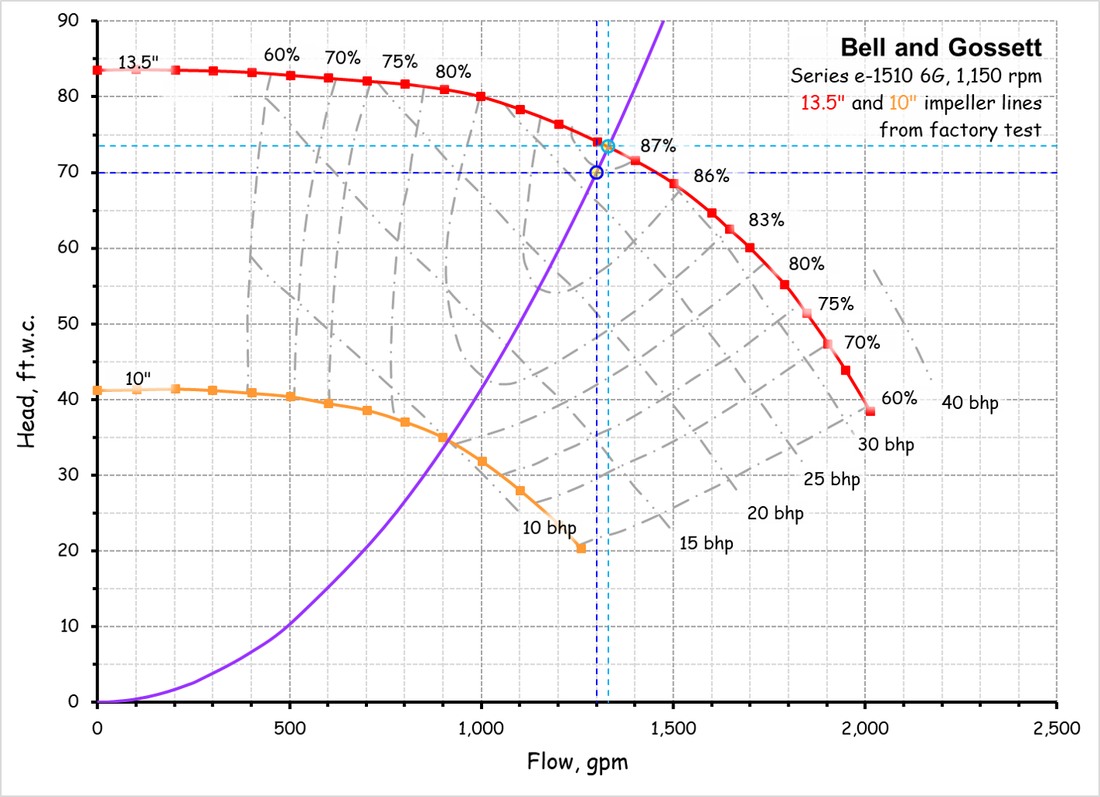
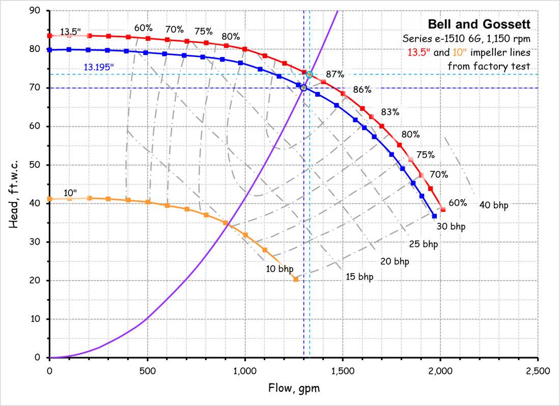
A Few General Affinity Law ConceptsThis affinity law allows you to project the flow that will be produced with a larger or smaller impeller given a known operating point on a known impeller line.
|
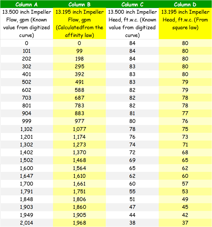
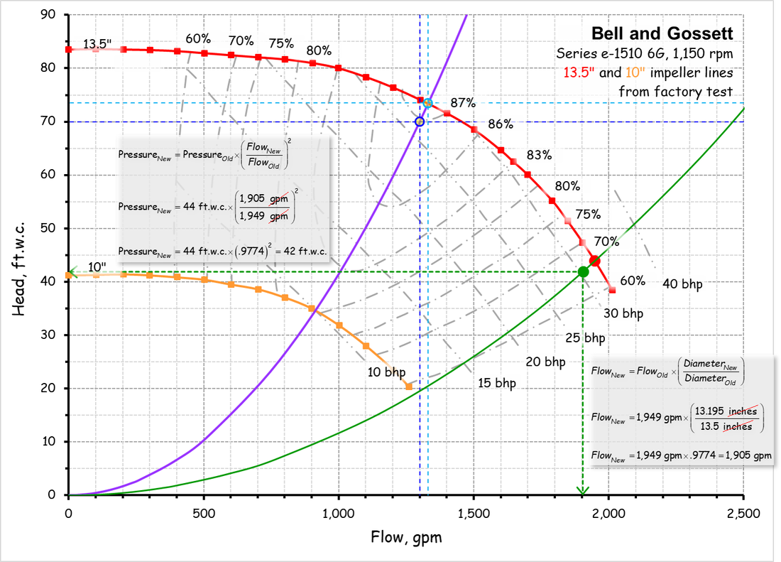
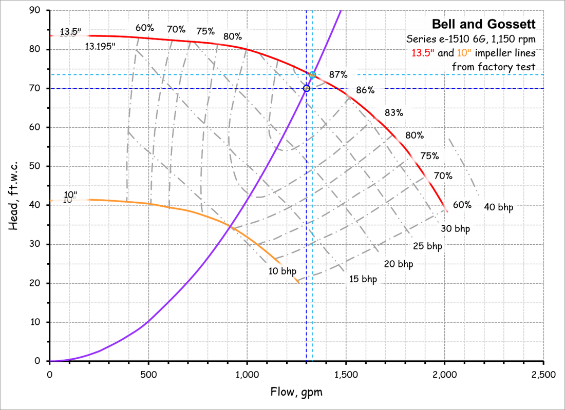
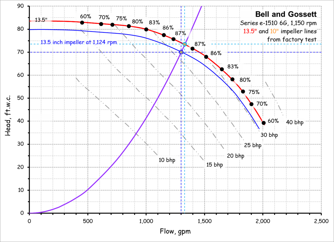
The Relationship Between Flow and Impeller DiameterThis affinity law allows you to project the flow that will be produced with a larger or smaller impeller given a known operating point on a known impeller line.
|
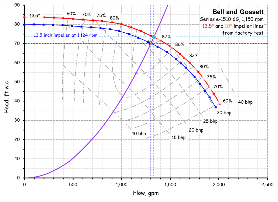
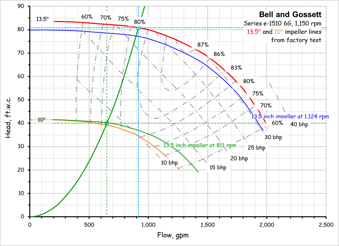
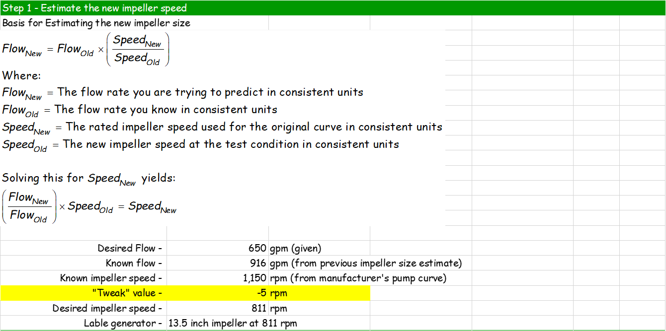
The Relationship Between Flow and Impeller SpeedThis affinity law allows you to project the flow that will be produced with a given impellers size operating at different speeds given a known operating point on the impeller line.
|
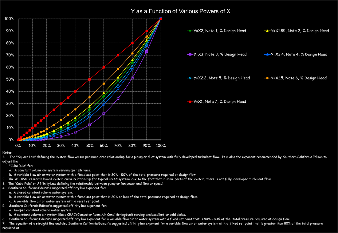
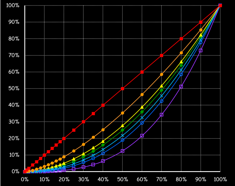
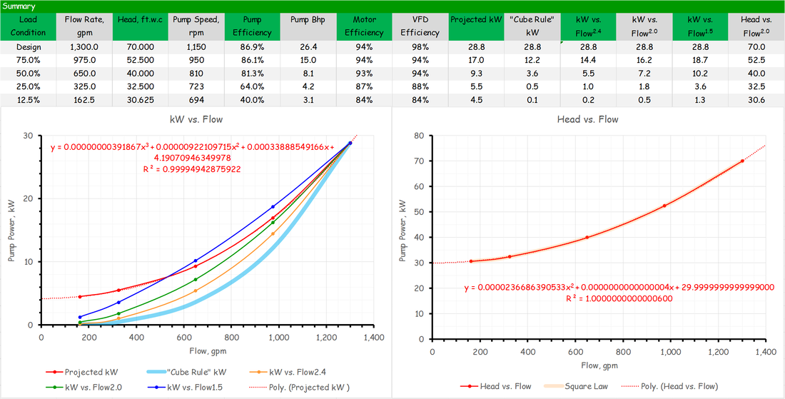
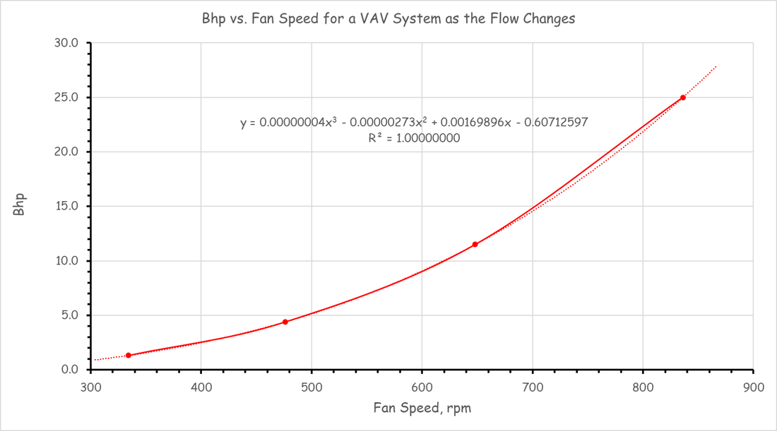
The Relationship Between Power and Impeller Speed; a.k.a "the Cube Rule"This affinity law allows you to project the power required by a given impeller size operating at a given speed relative to what it requires operating at a known speed and operating point on the impeller line. It is a cubic relationship and thus very powerful and attractive from an energy efficiency standpoint. But it is also frequently misapplied.
In addition to the affinity law, this section illustrates two different techniques that can be used to project energy consumption based on a system's flow profile. |
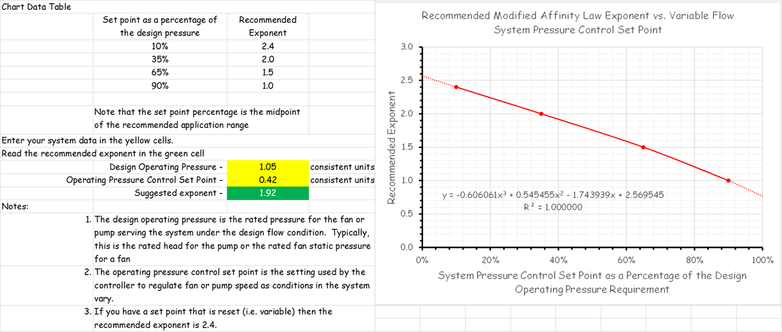
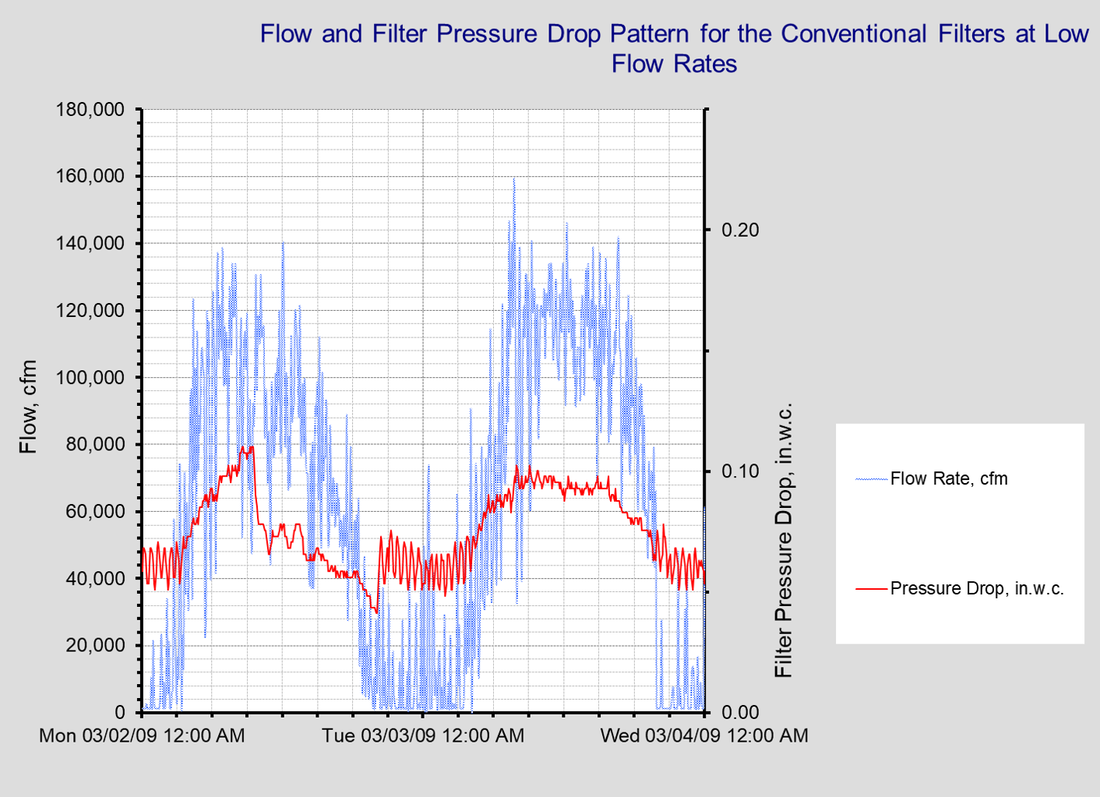
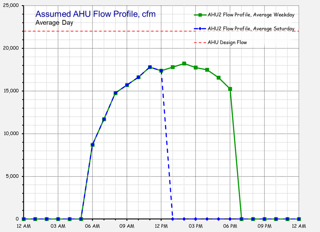
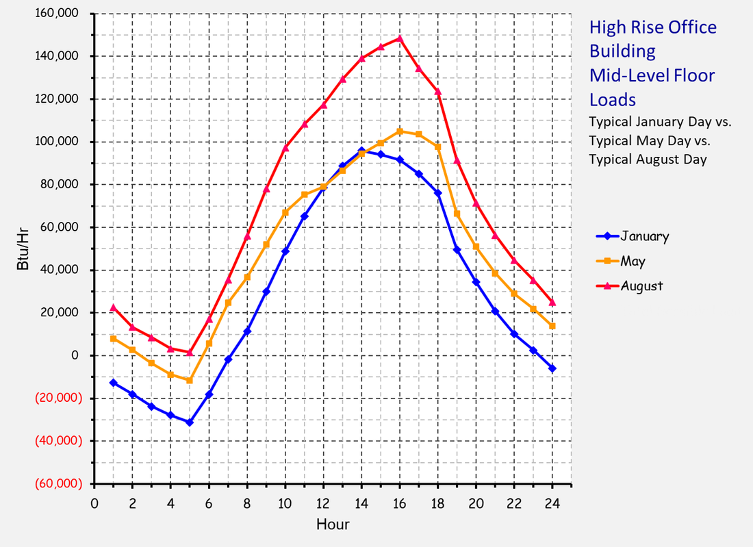
The Load Profile - A Key Element for Projecting Energy UseAs is discussed in the section about the cube rule, that law can be applied to project energy consumption for a fan or pumping system. But variable flow systems introduce several complexities and one is the need to have a load profile to work from. This section discusses some options for coming up with a load profile.
|
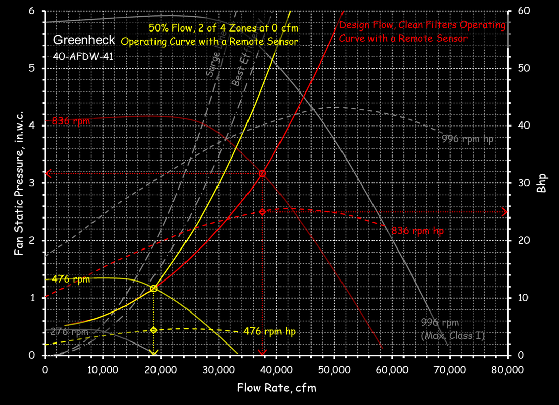
A Common Affinity Law MisapplicationFrequently, it is assumed that if there are two fans or pumps in parallel serving a load, the, via the cube rule, significant energy will be saved by operating both of the fans or pumps together at a lower speed as compared to operating a single fan or pump at a higher speed to serve the same load.
While this is true for some very specific cases (parallel independent cooling tower cells are a good example), it is generally not true. This section discusses the reason and provides some resources to further explain the fallacy. |