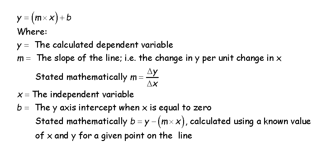
y = (m * x) + b SpreadsheetThe equation for a straight line makes frequent appearances in engineering calculations. One of the most common applications for me is to determine the relationship between the signal being generated by a transmitter and the data it represents.
|
|
For instance, if I have a temperature transmitter that generates a 4-20 ma output, going from 4 ma to 20 ma as the temperature varies from 0°F to 100°F, then I can use the equation of a straight line to calculate the temperature that is being measured currently by the transmitter based on the current I am reading on my meter. In fact, for many control systems and control devices, you are actually setting up this relationship in the device or system when you enter the zero and span parameters for a given data point or device.
A while ago, I decided that I was doing this often enough that I should take on of the spreadsheets I used to do it and make it into a little tool so that I didn't have to keep re-inventing the wheel. This web page gives you access to that spreadsheet.
A while ago, I decided that I was doing this often enough that I should take on of the spreadsheets I used to do it and make it into a little tool so that I didn't have to keep re-inventing the wheel. This web page gives you access to that spreadsheet.
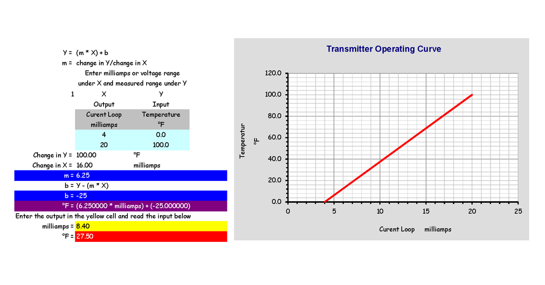
One tab on the spreadsheet allows you to enter the specifics for the transmitter you are working with and then illustrates the result in a graph. It also allows you to enter a current reading from your meter and calculates the associated input temperature based on the specifics of the transmitter. In the example, I have the spreadsheet set up for a 0-100 °F input and a 4-20 milliamp output. But you can edit the units of measure to be anything you want; i.e. 1-5 vdc, 2-10 vdc, 0-30 psig, 0.0 - 0.5 in.w.c., etc.
Frequently, when you are commissioning a transmitter like this out in the field, you are comparing what you are reading from the transmitter with some sort of reference standard to determine if the transmitter is properly calibrated. When doing this, it is important to remember that the indicated value, in the case of the example, 27.50°F, represents the output from a perfect transmitter/sensor assembly.
All real transmitters and sensors have an accuracy tolerance. For instance, if the tolerance for the transmitter in the example was +/- 2.5°F, as long as my more accurate reference standard said that the actual temperature at the time was between 27.50°F + 2.5°F or 30°F and 27.50°F - 2.5°F or 25°F, then the transmitter would be considered as meeting its accuracy specification.
To help me be able to visualize this, I added a tab to my spreadsheet tool that not only shows the theoretical line, it also shows the accuracy band for the transmitter.
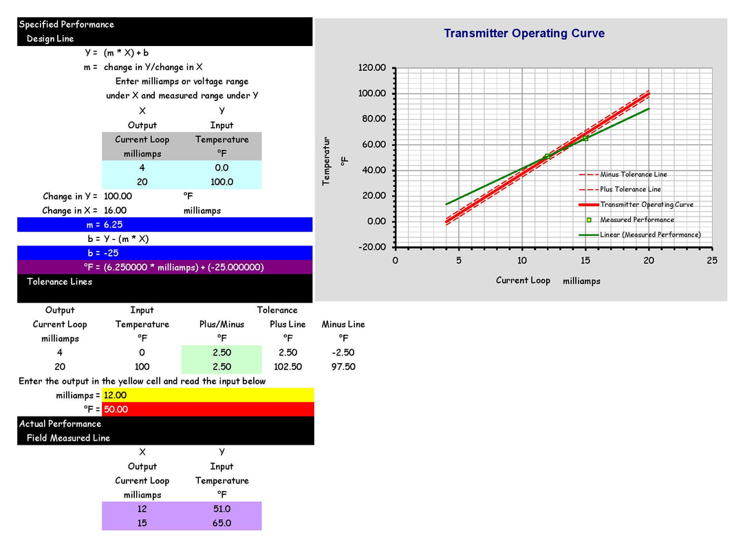
This allows me to see not only if the current point is with in the accuracy band associated with the device, but also if the transmitter will be accurate over its entire range. I can accomplish this by measuring a second point and plotting the line connecting the two points. If that line exits the accuracy band, I know the transmitter is not going to be accurate over its entire range and also which part of the range it will be accurate over.
The latter helps me decide how best to calibrate the transmitter. If I only require it to be accurate over a narrow band, then it may be sufficient to simply put in an offset, which shifts the current reading so that it is correct (essentially, it shifts the y intercept; this is the zero adjustment on a transmitter with a zero and span adjustment) but does not change the slope. This may be sufficient for a point that does not vary much in normal operation, and I don't care what the value is if the system is not in normal operation.
But if I need accuracy over the entire span of the transmitter, then I need to measure a second point, preferably as far away from the first measurement as possible, and then adjust the slope based on this measurement so that it falls inside the accuracy window over the entire span of the transmitter. This is the span adjustment on a transmitter with a zero and span adjustment. Often, the zero and span adjustment can be interactive so if you change one, you need to back-check the other to make sure it still is where you need it.
I have included a slide set you download along with the spreadsheet tool if you want to know more about one point vs. multi-point calibrations.
So far, i have illustrated how I use the spreadsheet in the context of the function I originally built it to support. But truth be told, you can use it to evaluate any function that is represented by a straight line. For example, the other day,. when I was checking logic associated with a reset schedule, I adjusted the units of measure to allow me to set it up to represent the reset schedule and calculate the output as a function of different inputs.
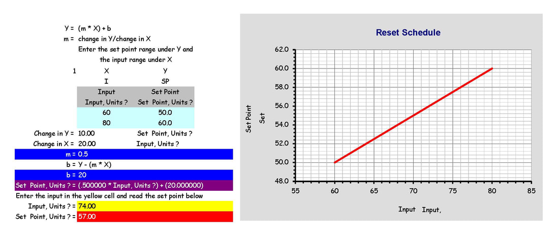
Note that the logic in this particular example had dimensionless inputs and outputs. A more conventional reset schedule, or instance, once that reset hot water supply temperature based on outdoor air temperature, would have engineering units for temperature associated with the input and output.
The links below should download the spreadsheet tool and the calibration slides. I have also included the .wmf and .pdf files that have the equation in them in case you want to illustrate the equation in a spreadsheet or other document. I explain a bit more about how to do that on the Useful Formulas home page of the web site.
May all of your lines be straight and your transmitters accurate.
|
| ||||||||