Insulation Savings ToolsA very low cost/no cost option for saving energy in steam and hot water systems is to simply repair insulation. But for insulation on things like control valves, the repair is less likely to persist because of the need to occasionally remove the insulation to perform service work.
Removable fitting covers offer an attractive alternative for insulating items that may require service down the road in new installations and as an alternative repair strategy for existing systems. |
|
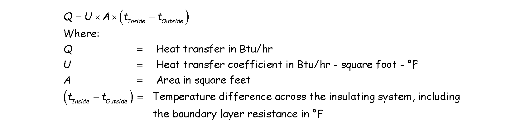
Of course, if you are need to justify the improvement or repair, you frequently need to provide an estimate of the savings that will be achieved by installing insulation or fitting covers. In general terms, the losses will be proportional to the thermal resistance of the insulation, the temperature difference, and the area of surface that is exposed and will now be insulated. The relationship is fairly straight forward and a very common form of the basic relationship that is used when assessing the losses through the walls of a building looks something like this.
That relationship has it's roots in Fourier's Law of heat conduction, which looks like this.
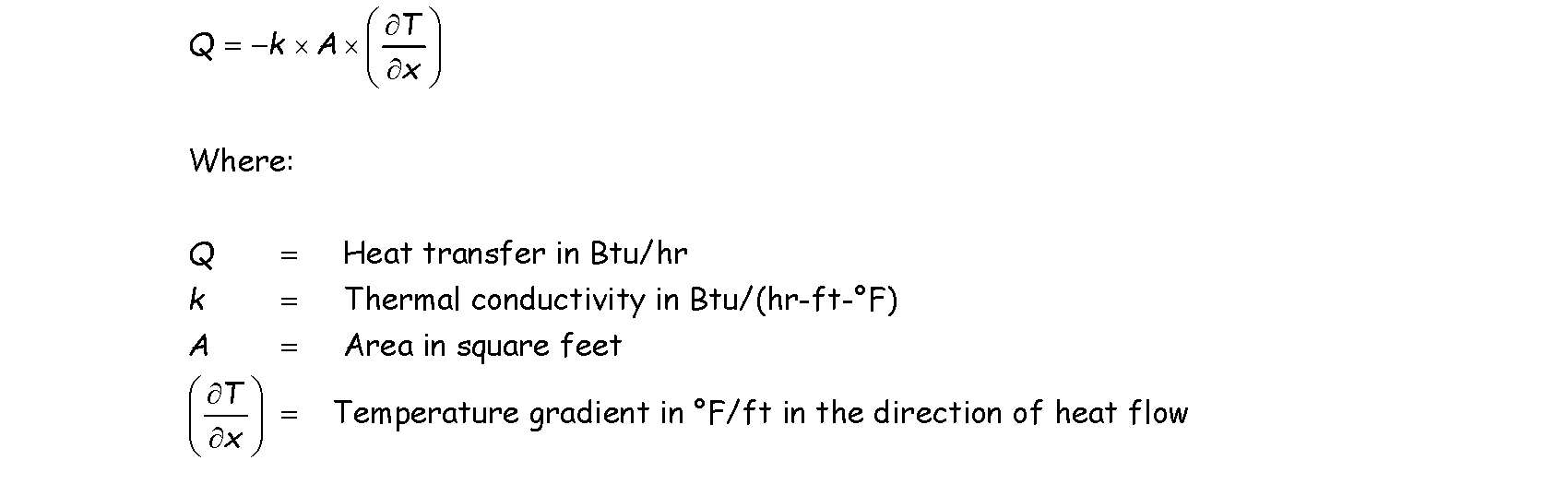
The negative sign ahead of k is to satisfy the law of thermodynamics that says heat must flow from warmer temperatures to cooler temperatures.
|
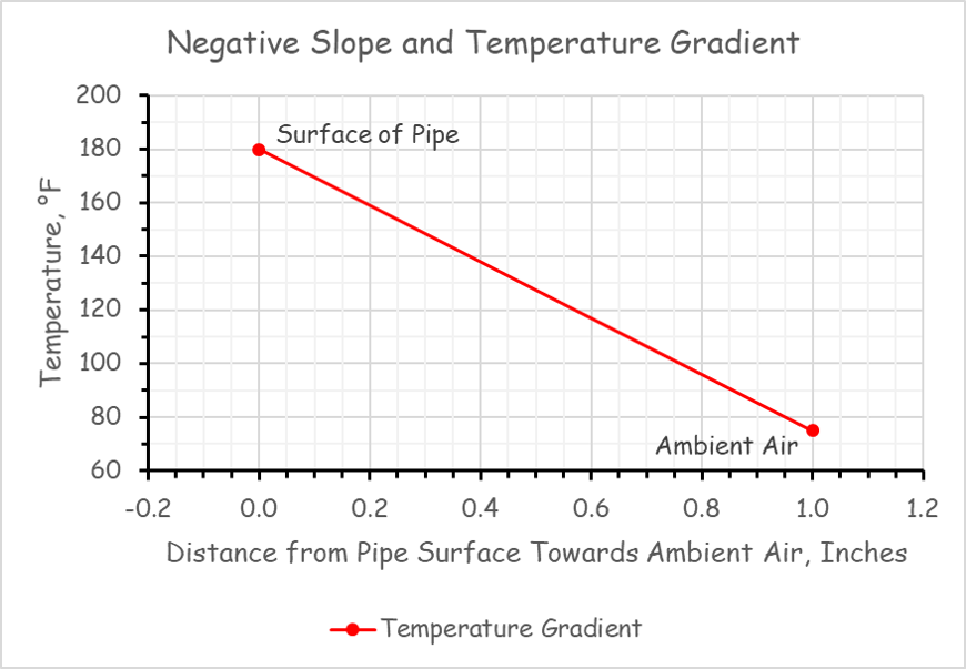
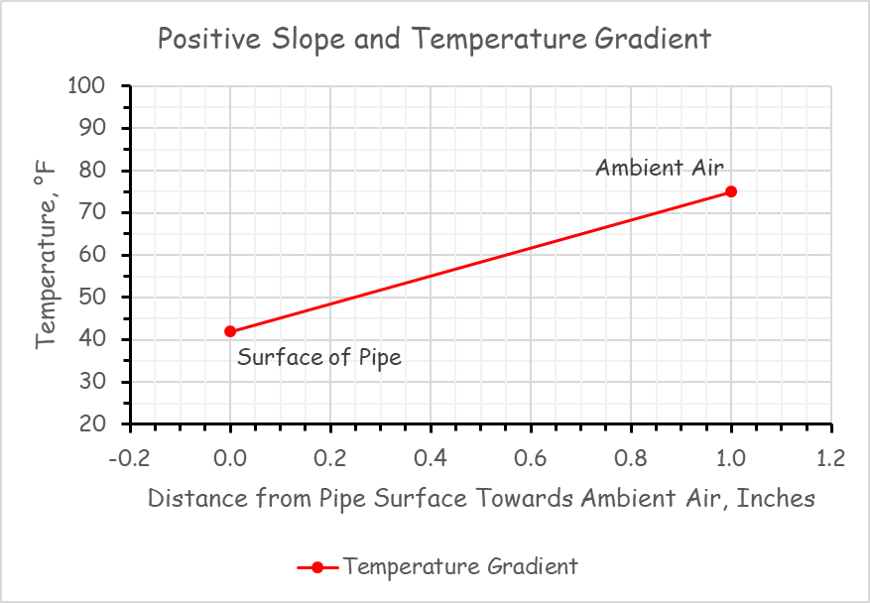
For example, if a hot surface had 1 inch of insulation covering it, and you plotted temperature vs. distances from the hot surface as you moved through the insulation, you would get a line that sloped from high on the left side to low on the right side assuming your coordinate system had temperature on the y axis with increasing temperature going up and distance on the x axis with increasing distance going right. (upper figure). In other words, as your distance from the hot side increased (the x value), the temperature at a given point would have decreased (the y value) relative to what it was at the hot surface.
The change in y relative to the change in x is termed the "slope" of the line and in mathematics, a line defined by a relationship where the y value decreases as the x value increases is said to have a negative slope. Since in our case, the change in y relative to the change in x is the thermal gradient, for the hot surface with insulation on it, the thermal gradient would be negative. For a cold pipe, the gradient would be the other way and would be a positive slope and gradient (lower illustration). |
As a result, when you evaluated the expression for a hot pipe, the heat transfer would be considered positive (negative k times a negative gradient gives a positive number); i.e. energy flowed away from the higher temperature area to the lower temperature area, which satisfies the thermodynamic law.
When you apply Fourier's law to something like a flat wall with a layer of insulation on it that is uniform and where the wall can be considered large enough that it is reasonable to assume that all of the energy is flowing perpendicular to the face of the wall, then when you integrate the equation, you end up with the very familiar relationship I started out with.
When you apply Fourier's law to something like a flat wall with a layer of insulation on it that is uniform and where the wall can be considered large enough that it is reasonable to assume that all of the energy is flowing perpendicular to the face of the wall, then when you integrate the equation, you end up with the very familiar relationship I started out with.
|
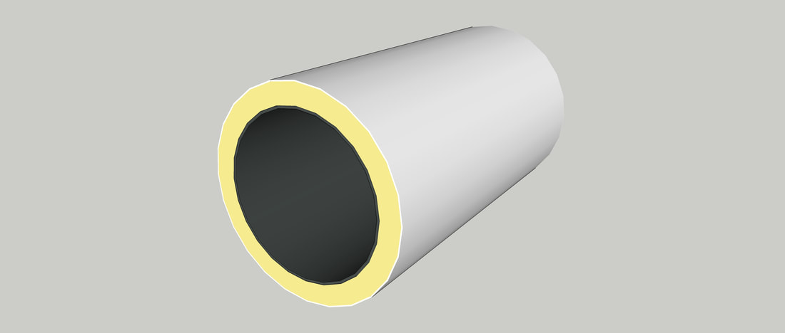
But when you apply Fourier's equation to a pipe, a complication comes up. Consider a 4 inch pipe that is at 180°F and is insulated with 1 inch of insulation and suspended in a 75°F space (top image).
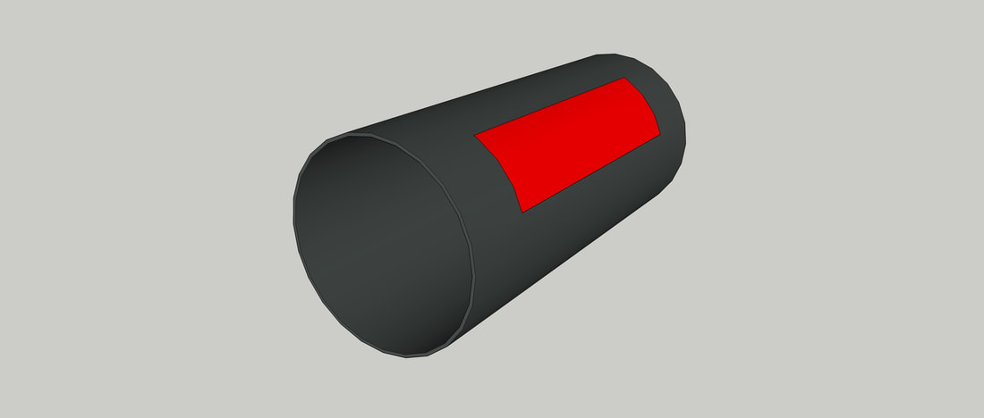
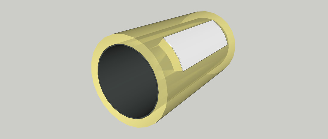
Let's remove the insulation and select an area of the pipe to study, specifically the area in red in the middle image. Energy leaving the pipe from the red area will flow radially outward through the insulation to the surrounding cooler space in accordance with the first law of thermodynamics. But because straight lines radiating from the center of the pipe diverge, the area that the energy flow passes through when when it leaves the insulation jacket to enter the space is larger than the area on the surface of the pipe. Specifically, the area of the red surface in the middle picture is about 35 square inches, but the area that you create when you project the for corners of the red rectangle radially out through the insulation (the white area in the bottom picture) is 47.5 square inches. The thicker the insulation is, the larger the difference in areas will be. |
As a result, when you integrate Fourier's equation to take into account how the area of the surface of a cylinder varies with radius, you end up with a much more intimidating looking equation.
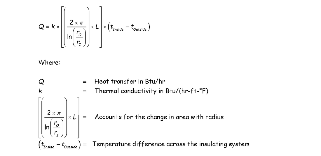
Plus to get the solution you have to apply calculus to perform and integration; pretty scary if you are math phobic, like me.
That's the bad news. The good news is that since estimating heat loss from pipes and ducts is a very common need, there are a lot of tools out there that can help you do it with math that is much less intimidating. And my purpose in adding this page to the web site is to put you in touch with some of them.
My purpose in exposing you to Fourier's Law is that I think it is important to understand where the principles you are applying come from so that you don't misapply a tool that has some simplifying assumptions built into it. For instance, one of the tools below is for estimating losses from insulated valves. If you thing about how much the shape of a valve varies and the implications regarding the area through which heat would need to flow to leave it, you quickly conclude that if you were to develop an equation to describe it, then it would be even more scary than the one for a cylinder.
I suspect (but don't know) that the tool is empirical, meaning the data was generated by taking measurements rather than by developing a lot of mathematics. But my point is that in realizing some of the issues that are behind the tool, you are less likely to abuse it. So for example, while the tool is focused on valves in steam systems, extrapolating it to valves in hot water systems is reasonable if you are careful about it. But extrapolating it to project the energy losses the body of a hot water pump might be starting to push the limits.
But on the other hand, since a the shape of most pumps could be generated by putting different sized cylinders together, you may be able to use the tools for estimating the losses from a pipe to estimate the loss from a pump by considering it as an assembly of cylinders, evaluating the loss from each cylinder, and then adding them up.
I suspect you get my drift and are just wishing I would tell you about the resources, so here they are.
|
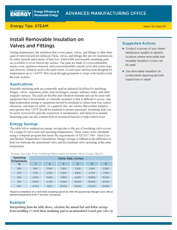
The Department of Energy publishes "tip sheets" for a number of energy using pieces of equipment and systems, including pumps, motors, compressed air systems, process heating systems and steam systems. Of interest in the context of this particular web page are the tip sheets for estimating the savings to be achieved by repairing steam pipe and valve insulation.
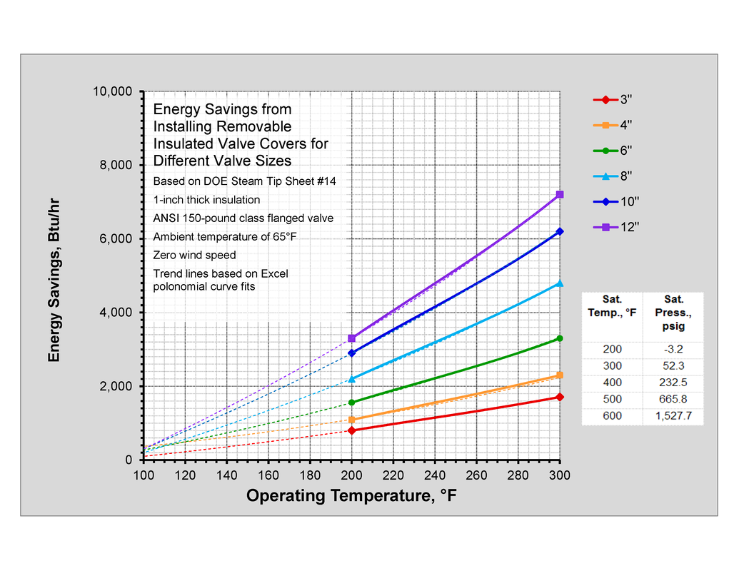
As you can see from the example to the left, the tip sheet takes all of the scary math out of the estimating process. Basically, if you can come up with the temperature that the valve is at (maybe "shoot" it with an infrared thermometer) and an estimate of the line size (maybe from a number on the casting or a diameter tape measure), then you can come up with the savings you could achieve by insulating the valve. For valve sizes and temperatures other than those listed in the table, you can do a simple linear interpolation between the values in the table. And, it is reasonable to assume that insulating valves in hot water systems would provide similar savings. However, hot water |
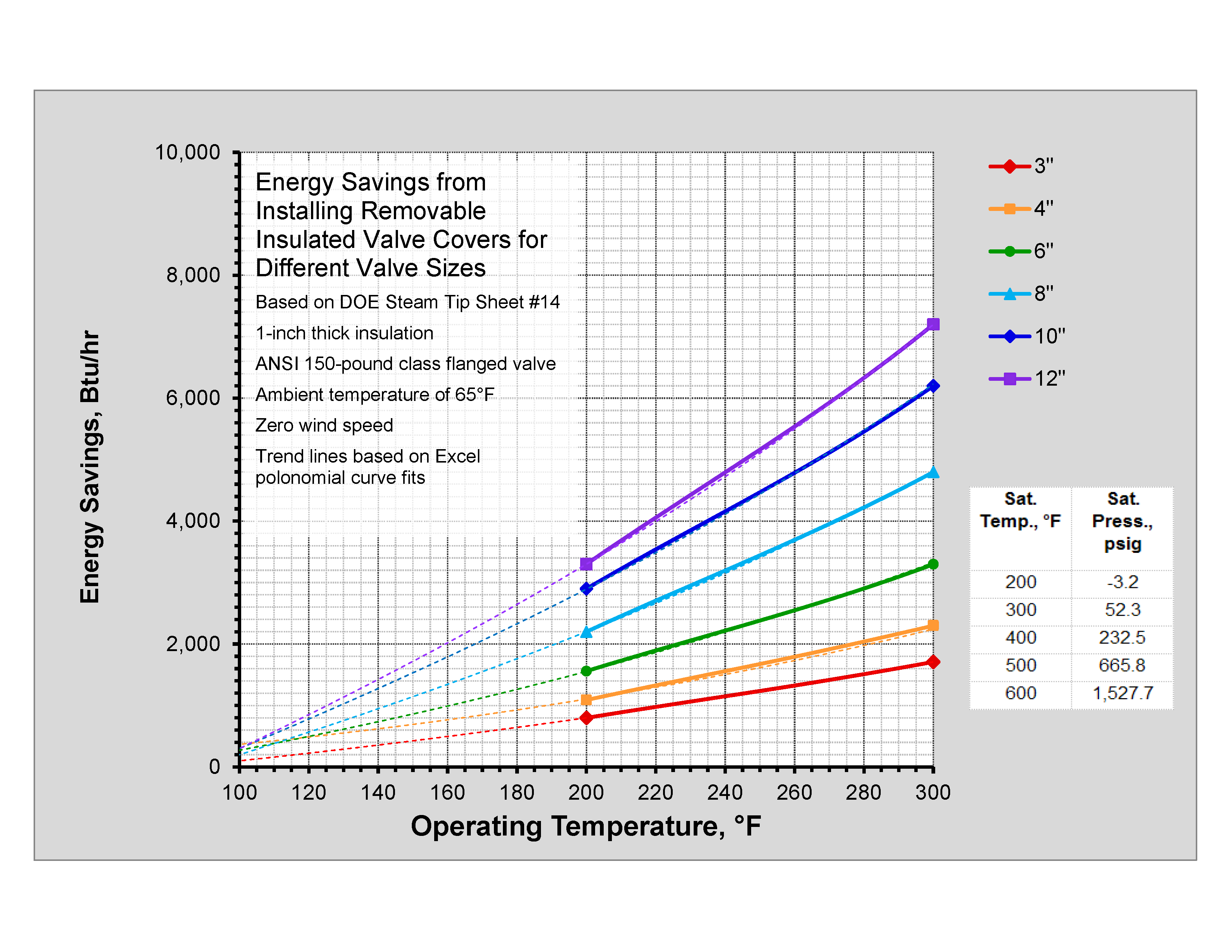
systems often operate at temperatures lower than the temperatures associated with steam systems meaning you need to extrapolate the data vs. interpolating it. But since the main driver for the heat transfer is the temperature difference across the insulation once you have taken the area into consideration, I concluded that it was reasonable to extrapolate the data from the table and project the losses for lower temperatures, which is what the chart at the top of the page illustrates.
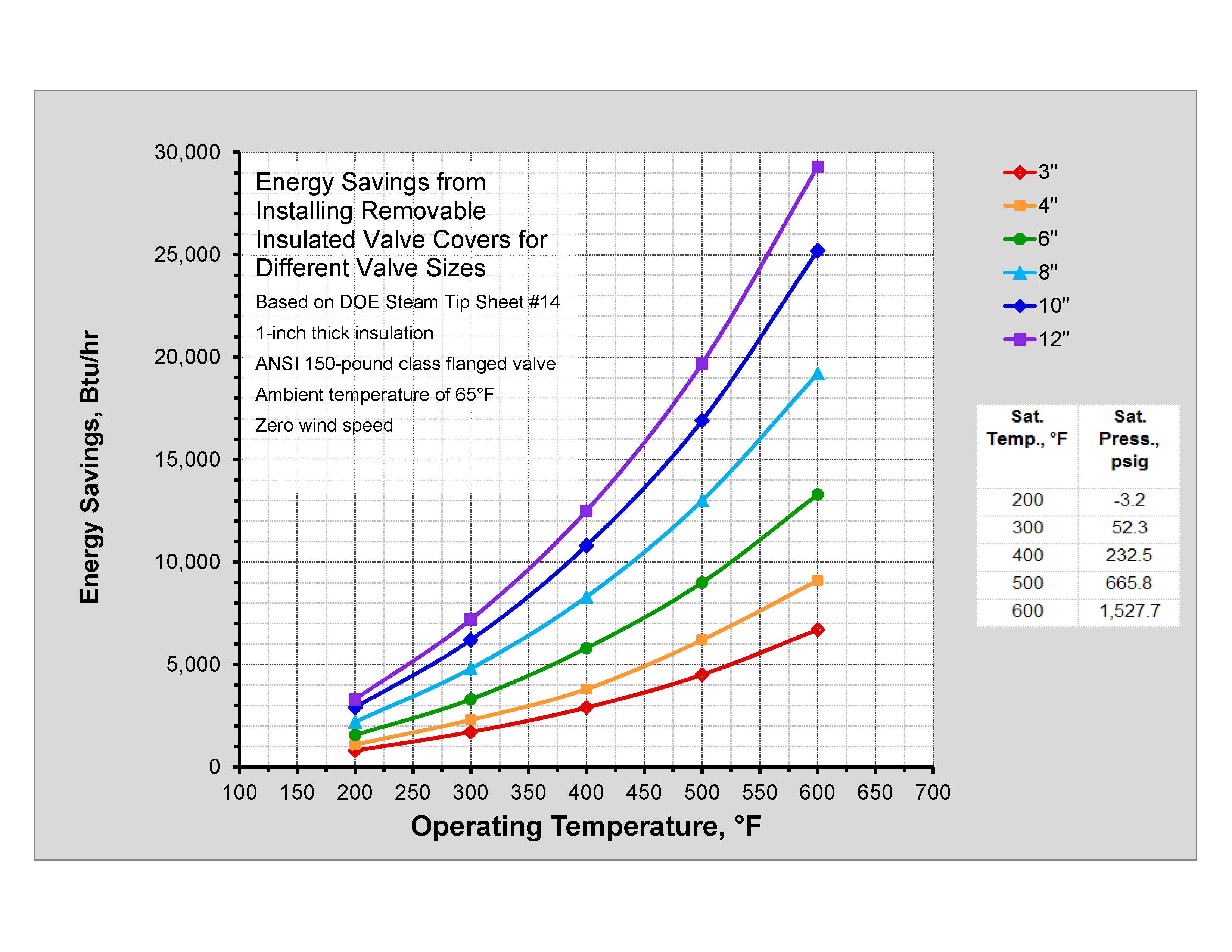
I created the chart by plotting the data in the table and then using Excel's trend line feature to project the losses at lower temperatures. I feel the projections are reasonable because they tend to converge at 0 Btu/hr as the temperature difference between the pipe and the surroundings approaches 0. Another benefit of the chart is that it lets you visually interpolate for values between the numbers in the table. So, I also made a chart that was derived by plotting the data in the table. The downloads below are both versions of the chart if you would like to use them and the spreadsheet behind them. The benefit of the spreadsheet is that it has some cells set up that allow you to fine tune your reading by moving a vertical and horizontal line around on the chart so that they cross exactly on the curve you are interested in.
I created the chart by plotting the data in the table and then using Excel's trend line feature to project the losses at lower temperatures. I feel the projections are reasonable because they tend to converge at 0 Btu/hr as the temperature difference between the pipe and the surroundings approaches 0. Another benefit of the chart is that it lets you visually interpolate for values between the numbers in the table. So, I also made a chart that was derived by plotting the data in the table. The downloads below are both versions of the chart if you would like to use them and the spreadsheet behind them. The benefit of the spreadsheet is that it has some cells set up that allow you to fine tune your reading by moving a vertical and horizontal line around on the chart so that they cross exactly on the curve you are interested in.
|
| ||||||
I should also point out that if you make your own spreadsheet and do the curve fits for the projections, the Excel trend line feature allows you to display the equation for the trend line. What that means is that you have a mathematical relationship that defines losses as a function of temperature for each of the line sizes.
So, if you were doing calculations that involved multiple rows in a spreadsheet (say an hour by hour savings assessment or a bin calculation), you could write a formula based on the trend line equation that would do the math for you instead of your needing to look up the number you need for each row or bin (which could get a bit tedious if you were doing an hour by hour calculation given that there are 8,760 hours in a year).
So, if you were doing calculations that involved multiple rows in a spreadsheet (say an hour by hour savings assessment or a bin calculation), you could write a formula based on the trend line equation that would do the math for you instead of your needing to look up the number you need for each row or bin (which could get a bit tedious if you were doing an hour by hour calculation given that there are 8,760 hours in a year).
|
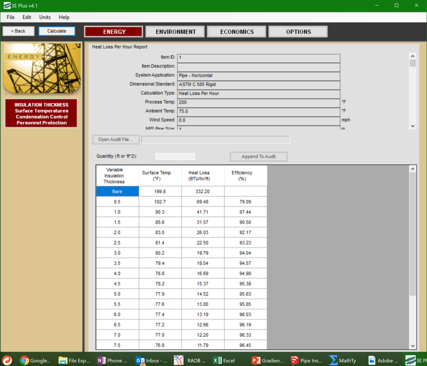
Finally, a discussion about ways to estimate savings associated with insulation would be totally incomplete if I did not mention the North American Insulation Manufacturer's Association software tool 3EPlus.
3EPlus allows you to quickly evaluate different insulation systems for a variety of applications including pipes, ducts, tanks, and flat surfaces. The screen shot to the left illustrates the results I generated for a 4 inch pipe operating at 200°F indoors in a 75°F environment and includes the losses for the bare pipe and different insulation thicknesses. The insulation was the typical fiberglass insulation you find in |
commercial applications but the tool includes numerous options and also allows you to build up a system using layers of different insulation. I generated the results faster than the time it took for you to read this. And I did not have to get out my calc book to look up an integration formula. But since I know the theory behind the tool and can spot check it with the equation for losses from a cylinder (above), I am pretty comfortable with the results with out doing the math myself.